ST-TS-HGR-NET

1 ST-TS-HGR-NET

ST-TS-HGR-Net: Spatial-Temporal and Temporal-Spatial Hand Gesture Recognition Network

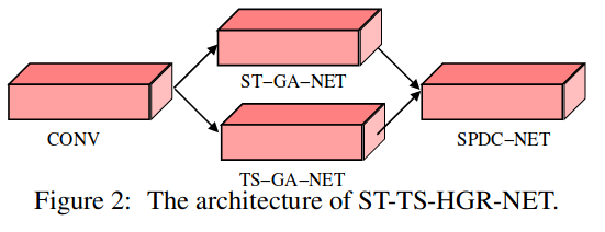
ST-TS-HGR-NET is a two-branch hand-gesture network that combines spatial-then-temporal and temporal-then-spatial Gaussian aggregation before learning a final SPD representation.

Ref: @nguyenNeuralNetworkBased2019

Code not available.

Overview

ST-TS-HGR-NET directly accepts sequences of 3-D hand-joint coordinates and contains three components:

1. CONV: shared per-frame spatial convolution over a hand-skeleton grid.
2. ST-GA-NET and TS-GA-NET: complementary Gaussian aggregation branches that encode first- and second-order statistics.
3. SPDC-NET: learned SPD aggregation, logarithmic mapping, vectorization, and classification.
   Unlike SPDNet, which receives a covariance matrix computed from a whole sequence, ST-TS-HGR-NET learns from raw joint coordinates, keeps mean as well as covariance information, and models separate fingers and temporal partitions at finer granularity.

Architecture

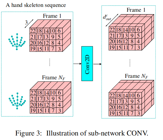
Spatial Convolution

The irregular hand skeleton is mapped to a 2-D grid with three channels for $x$, $y$, and $z$. Some joints are removed and additional cross-finger neighborhood connections are introduced. Each node has at most nine neighbors, including itself. For joint $i$ at frame $t$,

$$p_i^t=\sum _{j\in {\mathcal{N}}_i}{W}_{l(j,i)}{p}_{0,j}^t,$$

where $p_{0,j}^t\in {\mathbb{R}}^3$, ${\mathcal{N}}_i$ is the grid neighborhood, and one of nine shared weight matrices is selected by relative grid position. The same filters are shared across all frames.

Gaussian Embedding (GaussAgg)

To understand the SPDAgg layers, let us follow the authors’ explanation:

• Let $N_J$ and $N_F$ be respectively the number of hand joints and the length of the skeleton sequence. Let us denote by ${\mathbf{p}}_{0,i}^t\in {\mathbb{R}}^3,i=1,\dots ,N_J,t=1,\dots ,N_F$, the 3D coordinates of hand joint $i$ at frame $t$.
• Let $d_{out}^c$ be the output dimension of the convolutional layer.
• Let us denote by ${\mathbf{p}}_i^t\in {\mathbb{R}}^{d_{out}^c},i=1,\dots ,N_J,t=1,\dots ,N_F$, the output of the convolutional layer. The output feature vector at node i is computed as:

$${\mathbf{p}}_i^t=\sum _{j\in {\mathcal{N}}_i}{\mathbf{W}}_{l(j,i)}{\mathbf{p}}_{0,j}^t$$

where ${\mathcal{N}}_i$ is the set of neighbors of node $i$, ${\mathbf{W}}_{l(j,i)}$ is the filter weight matrix.

• To aggregate features in a branch associated with sub-sequence $s$ and finger $f$, $s=1,\dots ,6,f=1,\dots ,5$, each frame of sub-sequence $s$ is processed through 4 layers.
• Let $J_f$ be the set of hand joints belonging to finger $f$, $t_b^s,t_e^s$ be the beginning and ending frames of sub-sequence $s$, $t$ a given frame of sub-sequence $s$, $\{{\mathbf{p}}_{s,j}^i|j\in {\mathbf{J}}_f,i=t_b^s,\dots ,t_e^s\}$ the subset of output feature vectors of the convolutional layer fed to the branch.
• Consider a sliding window $\{t-t_0,\dots ,t+t_0\}$ centered on frame $t$. Following previous works, ${\mathbf{p}}_{s,j}^i$ are assumed i.i.d. samples from a Gaussian distribution:

$$\mathcal{N}(\mathbf{p};{\mathbf{\mu }}_{s,f}^t,{\mathbf{\Sigma }}_{s,f}^t)=\frac{1}{|2\pi {\mathbf{\Sigma }}_{s,f}^t{|}^{\frac{1}{2}}}\exp \left(-\frac{1}{2}(\mathbf{p}-{\mathbf{\mu }}_{\mathbf{s},\mathbf{f}}^{\mathbf{t}}{)}^T({\mathbf{\Sigma }}_{s,f}^t{)}^{-1}(\mathbf{p}-{\mathbf{\mu }}_{s,f}^t)\right),$$

with parameters estimated as

$${\mathbf{\mu }}_{s,f}^t=\frac{1}{(2t_0+1)|J_f|}\sum _{j\in {\mathbf{J}}_f}\sum _{i=t-t_0}^{i=t+t_0}{\mathbf{p}}_{s,j}^i,$$ $${\mathbf{\Sigma }}_{s,f}^t=\frac{1}{(2t_0+1)|J_f|}\sum _{j\in {\mathbf{J}}_f}\sum _{i=t-t_0}^{i=t+t_0}({\mathbf{p}}_{s,j}^i-{\mathbf{\mu }}_{s,f}^t)({\mathbf{p}}_{s,j}^i-{\mathbf{\mu }}_{s,f}^t{)}^T,$$

• Based on the method in @lovricMultivariateNormalDistributions2000 that embeds the space of Gaussians in the Riemannian symmetric space, the Gaussian can be identified as a SPD matrix given by:

$${\mathbf{Y}}_{s,f}^t=\left[\begin{array}{cc}{\mathbf{\Sigma }}_{s,f}^t+{\mathbf{\mu }}_{s,f}^t({\mathbf{\mu }}_{s,f}^t{)}^T& {\mathbf{\mu }}_{s,f}^t\\ ({\mathbf{\mu }}_{s,f}^t{)}^T& 1\end{array}\right].$$

• The GaussAgg layer performs this computation:

$${\mathbf{Y}}_{s,f}^t=h_{ga}(\{{\mathbf{p}}_{s,f}^t{\}}_{j\in {\mathbf{J}}_f}^{i=t-t_0,\dots ,t+t_0}).$$

This representation preserves both first-order and second-order statistics.

Branch Design

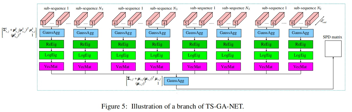
Each sequence yields six temporal selections: the complete sequence, two halves, and three thirds. Pairing these with five fingers gives 30 branches in ST-GA-NET and 30 branches in TS-GA-NET.

• ST branch: for each subsequence/finger/frame, the first GaussAgg aggregates every joint of that finger over the sliding window; the SPD matrix passes through ReEig → LogEig → VecMat (which preserves the Frobenius inner product by multiplying off-diagonal upper-triangular entries by $\sqrt{2}$). A second GaussAgg then aggregates these vectors over all frames of the subsequence, producing an SPD matrix that describes the temporal variation of finger $f$ within subsequence $s$.
• TS branch: each subsequence is divided into $N_S$ equal temporal pieces. For every joint and piece, the first GaussAgg computes an SPD matrix from that joint’s temporal samples; after ReEig → LogEig → VecMat, the second GaussAgg aggregates the vectors jointly over temporal pieces and the joints of finger $f$. This reverses the aggregation order: temporal statistics first per joint, then spatial pooling over the finger.

SPD Aggregation and Classification

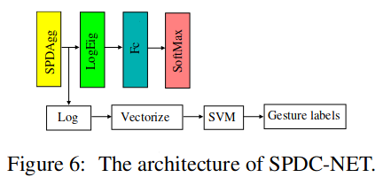
The 60 branch outputs are fused by SPDAgg:

$$Y=h_{\mathrm{spda}}((X_1,\dots ,X_N);W_1,\dots ,W_N)=\sum _{i=1}^N{W}_i{X}_i{W}_i^{\top }=\hat{W}\mathrm{diag}(X_1,\dots ,X_N){\hat{W}}^{\top },$$

with $\hat{W}=[W_1,\dots ,W_N]$. Positive definiteness follows when $\hat{W}$ has full row rank; it is constrained to the compact Stiefel manifold $\mathrm{St}(d_{\mathrm{out}}^s,N{d}_{\mathrm{in}}^s)$ and updated by projected gradient descent followed by retraction. The tail is SPDAgg → LogEig → upper-triangular vectorization (off-diagonals ×$\sqrt{2}$), and the reported final classifier is a LIBLINEAR SVM.

Model Parameters

• Spatial-convolution output dimension: $d_{\mathrm{out}}^c=9$; maximum grid neighborhood: 9 nodes.
• Temporal selections per sequence: 6; fingers: 5; branches: 30 + 30 = 60.
• Sliding-window radius $t_0=1$ (3 consecutive frames); TS subdivisions $N_S=15$; sequences normalized to $N_F=500$ frames.
• First GaussAgg: 9-D vectors → $10\times 10$ SPD; VecMat → 55 features; second GaussAgg → $56\times 56$ SPD.
• SPDAgg: input $d_{\mathrm{in}}^s=56$, output $d_{\mathrm{out}}^s=200$; each transformation matrix $200\times 56$.
• ReEig threshold: $ϵ=0.0001$.
• DHG input: 22 hand joints; FPHA input: 21 hand joints (no palm).

Training Parameters

• Batch size: 30.
• Learning rate: 0.01.
• Selected network checkpoint: epoch 15.
• Optimizer name, momentum, weight decay: not reported.
• SVM: LIBLINEAR L2-regularized L2-loss dual; $C=1$; stopping tolerance 0.1; no bias term.
• Implementation: MATLAB R2015b CPU; FPHA ≈22 min per training epoch and 7 min per test epoch.
• Frame counts 300/500/800 tested; differences marginal.

Results

Main results (accuracy %):

Dataset/protocol	ST-TS-HGR-NET	SPDNet
DHG, fixed split, 14 gestures	94.29	75.24
DHG, fixed split, 28 gestures	89.40	69.64
DHG, LOSO, 14 gestures	87.3	-
DHG, LOSO, 28 gestures	83.4	-
FPHA	93.22	84.35

Gains over SPDNet: +19.05 / +19.76 pp (fixed DHG 14/28) and +8.87 pp (FPHA). FPHA baselines: Gram Matrix 85.39, Lie Group 82.69, LSTM 80.14, ST-GCN 81.30, Grassmann network 77.57.

Ablations (FPHA / DHG-14 / DHG-28):

Ablation	FPHA	DHG-14	DHG-28
ST-HGR-NET only	91.83	93.21	89.29
TS-HGR-NET only	90.96	93.33	88.21
Full ST-TS-HGR-NET	93.22	94.29	89.40
3 neighbors (physical)	91.65	93.10	88.33
9 neighbors (augmented grid)	93.22	94.29	89.40
$t_0=1$	93.22	94.29	89.40
$t_0=2$	93.04	94.17	89.04
$t_0=3$	93.04	94.29	89.40
$N_S=15$	93.33	94.29	89.40
$N_S=20$	92.87	94.05	88.93
$N_S=25$	92.70	94.29	89.04