Tensor-CSPNet

1 Tensor-CSPNet

Tensor-CSPNet is a geometric deep-learning framework that represents temporally and spectrally segmented MI-EEG trials as tensors of spatial covariance matrices and learns CSP-like spatial filters on the SPD manifold.

Date of publication: 23/09/2022

Ref: @juTensorCSPNetNovelGeometric2022

Source code: https://github.com/GeometricBCI/Tensor-CSPNet-and-Graph-CSPNet

Overview

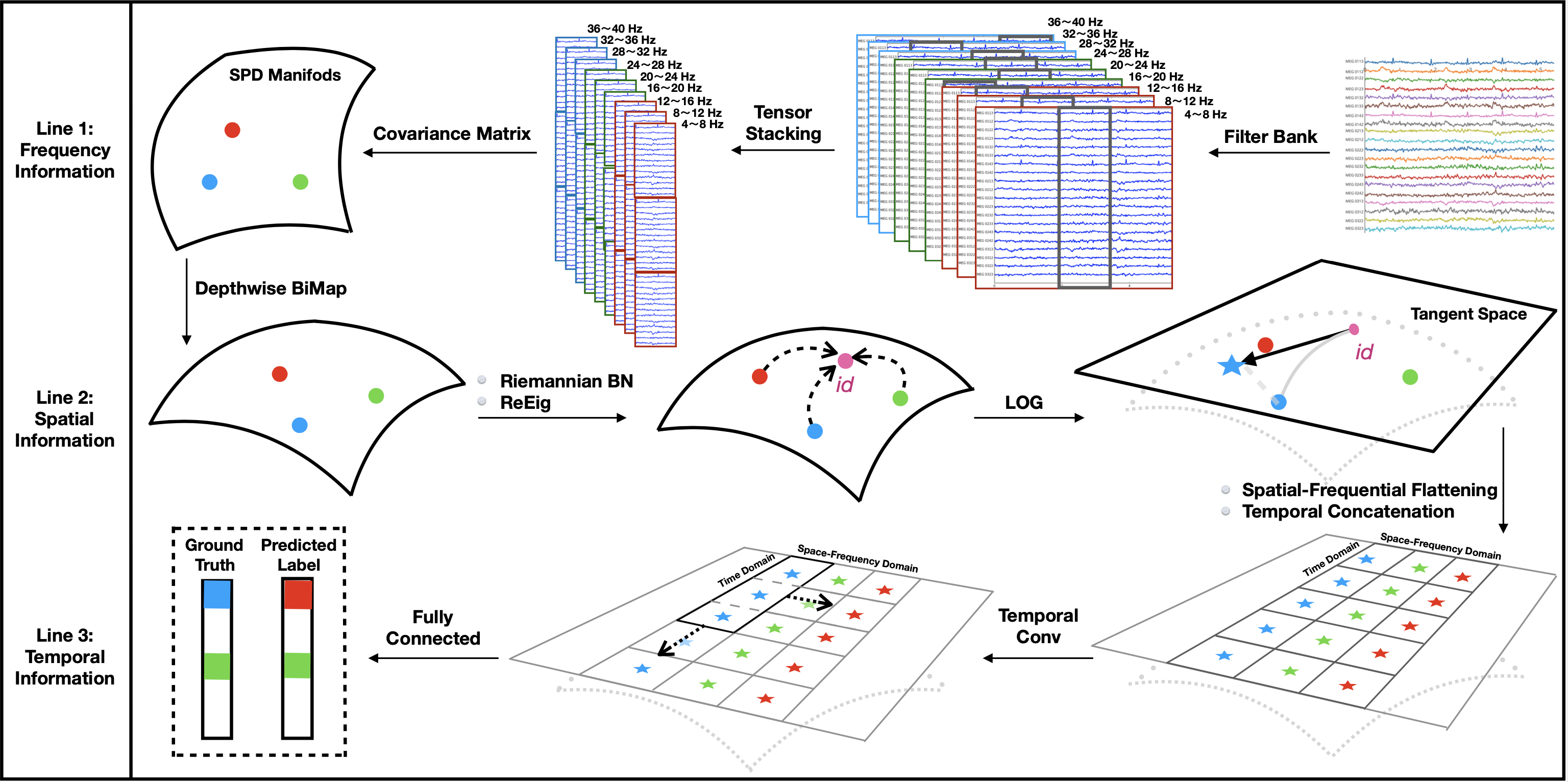
Tensor-CSPNet has four stages: tensor stacking, a common spatial pattern stage on SPD matrices, temporal convolution in tangent space, and classification.

• Datasets: Korea University Dataset (MI-KU/OpenBMI) and BCI Competition IV Dataset 2a.
• MI-KU: 54 subjects, two binary-MI sessions, 200 trials per subject per session, 62 electrodes at 1,000 Hz; 20 motor-cortex electrodes selected.
• BCIC-IV-2a: 9 subjects, 22 EEG + 3 EOG channels, 250 Hz, four classes, 288 trials per session.
• Frequency preprocessing: nine causal Chebyshev Type-II band-pass filters covering {4-8, 8-12, …, 36-40 Hz}. The method assumes trials are already band-pass filtered, centered, and scaled.
• Evaluation: subject-specific shuffled 10-fold CV within each session and cross-session holdout, S1→S2 for MI-KU and T→E for BCIC-IV-2a.

Temporal windows:

Model	Windows relative to the analyzed interval
MI-KU 1-CSPNet	{1.0-3.5 s}
MI-KU 5-CSPNet	{1.0-1.5, …, 3.0-3.5 s} (0.5 s)
MI-KU 10-CSPNet	ten non-overlapping 0.25 s windows from 1.00-3.50 s
2a 1-CSPNet	{0-4 s}
2a 3-CSPNet	{0-2, 1-3, 2-4 s}
2a 5-CSPNet	{0-2, 0.5-2.5, 1-3, 1.5-3.5, 2-4 s}
2a 7-CSPNet	seven overlapping 1-s windows from 0-4 s, 0.5 s stride

Architecture

For a trial $X\in {\mathbb{R}}^{C\times T}$:

1. Tensor stacking: filter-bank and temporal segmentation produce $\tilde{X}\in {\mathbb{R}}^{W\times F\times C\times \omega }$. A CovLayer-like operation forms one channel covariance per window and frequency: $S_{ij}=\tilde{X}[i,j,:,:]\tilde{X}[i,j,:,:{]}^{\top }$. BCIC-IV-2a commonly enters the network as a tensor of $22\times 22$ SPD matrices; MI-KU uses $20\times 20$.
2. CSP stage: a depthwise BiMap applies an independently learned congruence transform to each window-frequency covariance: $S_{ij}^{\prime }=W{S}_{ij}{W}^{\top }$. Unlike ordinary SPDNet BiMap, the depthwise operation does not sum channels after multiplication. It is followed by Riemannian batch normalization, ReEig, and LogEig.
3. Temporal convolution: after LogEig, frequency-space features are flattened and concatenated in temporal order; a 2-D CNN learns temporal dynamics in the Euclidean tangent space.
4. Classification: one- or three-layer fully connected networks with cross-entropy.

The CSP connection is explicit: BiMap learns a data-driven spatial projection rather than obtaining CSP filters through simultaneous diagonalization. Riemannian batch normalization acts analogously to regularized CSP, while ReEig turns the linear spatial filter into a nonlinear SPD-manifold transformation.

Model Parameters

The notation $w$-CSPNet$(m,n,l)@(p,q,r)$ means:

Parameter	Meaning	Values investigated
$w$	temporal windows	{1,5,10} MI-KU; {1,3,5,7} 2a
$m$	filter-bank channels	9
$n$	CSP blocks	{1,3}
$l$	FC depth	{1,3}
$o$	depthwise-BiMap output dim	{4,8,12,16,20,22,24,28,32,36}
$p$	temporal-CNN width factor	{1,9}
$q$	temporal-CNN height	$1\le q\le W$
$r$	temporal-CNN output channels	incl. {1,10,20}

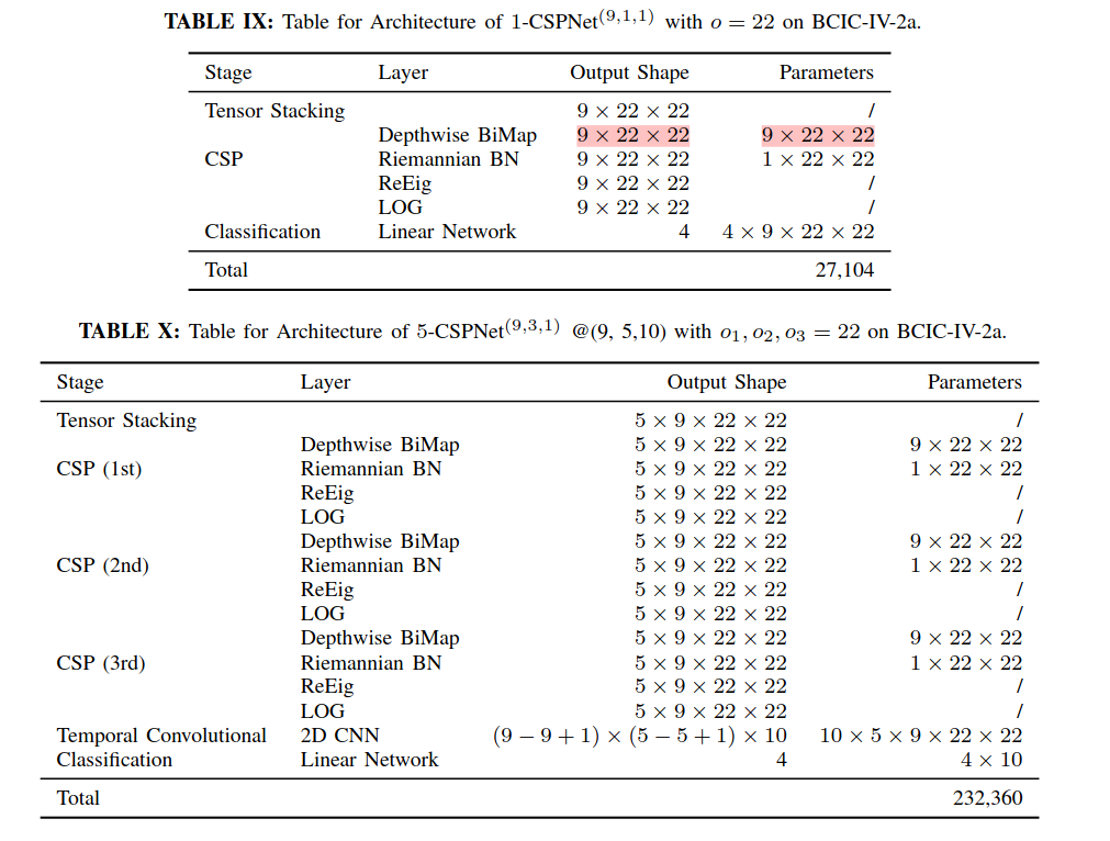
Main configurations: CV on both datasets 5-CSPNet(9,1,1); MI-KU holdout 10-CSPNet(9,1,1)@(9,5,2) with $o=20$; 2a holdout 5-CSPNet(9,1,1)@(9,5,4) with $o=22$. A 2a 1-CSPNet(9,1,1) with $o=22$ has 27,104 trainable parameters; a 5-CSPNet(9,3,1)@(9,5,10) with $o_1=o_2=o_3=22$ has 232,360 parameters. ReEig threshold: not reported.

Training Parameters

• Objective: cross-entropy.
• Initial learning rate: 0.01, with decay.
• Batch size: 28 (stated to equal the test-set size in the calibration-time experiment; note an MI-KU CV fold has 20 trials, and no MI-KU-specific batch size is reported — see Korea University Dataset (MI-KU or Lee2019 or OpenBMI)).
• Maximum epochs: 60; early stopping patience: 15.
• Optimizer: not reported.

MI-KU temporal-CNN height ($q$) ablation (accuracy): 5-CSPNet $q=\mathrm{1..5}$: 0.635, 0.651, 0.660, 0.668, 0.676; 10-CSPNet $q=\mathrm{6..10}$: 0.668, 0.674, 0.678, 0.672, 0.684.

Results

Average accuracy (%) with SD in parentheses:

Method	MI-KU CV S1	MI-KU CV S2	MI-KU S1→S2	2a CV T	2a CV E	2a T→E
FBCSP	64.41 (16.28)	66.47 (16.53)	59.67 (14.32)	73.57 (15.13)	72.46 (16.02)	65.79 (14.21)
MDM	50.47 (8.63)	51.93 (9.79)	52.33 (6.74)	62.96 (14.01)	59.49 (16.63)	50.74 (13.80)
TSM	54.59 (8.94)	54.97 (9.93)	51.65 (6.11)	68.71 (14.32)	63.32 (12.68)	49.72 (12.39)
SPDNet	57.88 (8.68)	58.88 (8.68)	60.41 (12.13)	65.91 (10.31)	61.16 (10.50)	55.67 (9.54)
EEGNet	63.35 (13.20)	64.86 (13.05)	63.28 (11.56)	69.26 (11.59)	66.93 (11.31)	60.31 (10.52)
ConvNet	64.21 (12.61)	62.84 (11.74)	61.47 (11.22)	70.42 (10.43)	65.89 (12.13)	57.61 (11.09)
FBCNet	74.16 (12.60)	73.81 (13.99)	67.83 (14.34)	77.26 (14.82)	76.58 (13.09)	72.71 (14.67)
Tensor-CSPNet	74.95 (15.27)	75.92 (14.63)	69.65 (14.97)	75.98 (14.26)	74.92 (14.63)	72.96 (14.98)

Selected ablations on BCIC-IV-2a CV: at $o=22$, 1-CSPNet(9,1,1) 0.7304 ± 0.1306, +Riemannian BN 0.7383 ± 0.1276; 1-CSPNet(9,3,3) 0.6945 → 0.7241 with BN. BiMap dimension sweep: 0.5793 at $o=4$ → 0.7496 at $o=36$ (0.7508 with BN). Without temporal convolution, 1/3/5/7-window variants score 0.7383 / 0.7238 / 0.7334 / 0.6821. Calibration time: 1-CSPNet(9,1,1)_BN 1,997.23 s; 5-CSPNet(9,1,1)_BN@(1,2,20) 8,860.63 s per subject.

Notes and Caveats

• Riemannian BN improved average accuracy by up to ≈1 pp in paired configurations, but the differences were not statistically significant.
• BiMap dimensional expansion sometimes outperformed dimensional reduction, contrary to the usual SPDNet interpretation of BiMap as only a compression layer.
• Signal normalization after filtering is not explicitly reported.