1 TSMNet

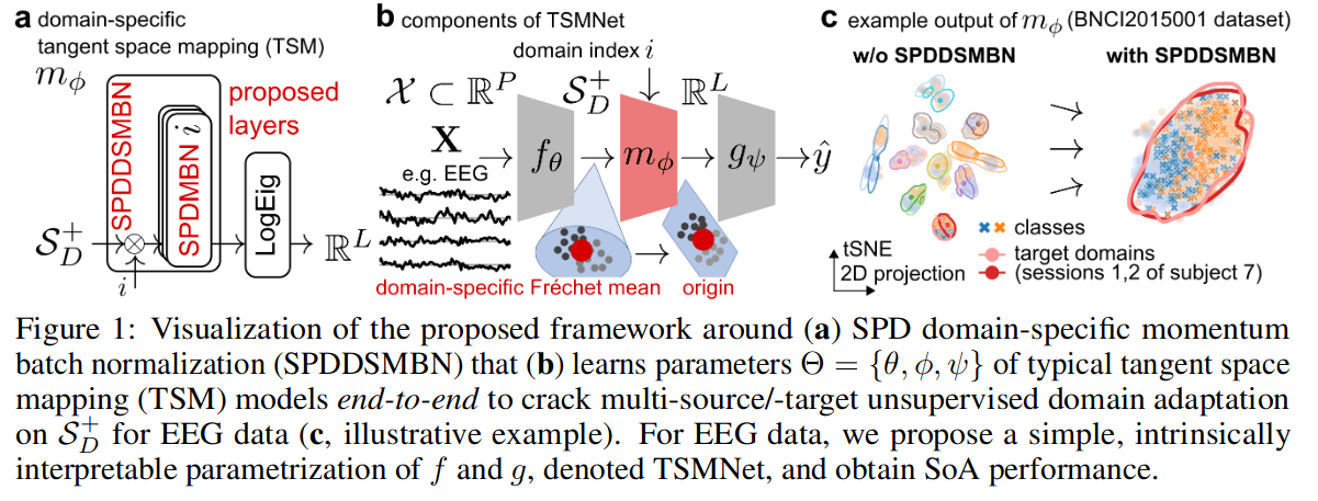
TSMNet is an interpretable end-to-end tangent-space EEG model whose SPD domain-specific momentum batch normalization aligns session- or subject-specific covariance distributions without target labels.

Date of publication: 12/10/2022

Ref: @koblerSPDDomainspecificBatch2022

Source code: https://github.com/rkobler/TSMNet

SPDDSMBN: SPD domain-specific momentum batch normalization

Overview

TSMNet addresses multi-source/multi-target unsupervised domain adaptation for EEG by maintaining domain-specific normalization statistics on the SPD manifold. The six motor-imagery datasets:

Dataset	Epoch	Rate	Channels	Subjects	Sessions	Classes
BNCI2014001 (BCI Competition IV Dataset 2a)	0.5-3.5 s	250 Hz	22	9	2	4
BNCI2015_001	1.0-4.0 s	256 Hz	13	12	2–3	2
Lee2019 (Korea University Dataset (MI-KU or Lee2019 or OpenBMI))	1.0-3.5 s	250 Hz	20	54	2	2
Stieger2021	1.0-3.0 s	250 Hz	34	62	4–88	4
Lehner2021	0.5-2.5 s	250 Hz	60	1	7	2
Hehenberger2021	1.0-3.0 s	250 Hz	32	1	26	4

Plus the three-class Hinss2021 mental-workload dataset: 0–2 s, 250 Hz, 30 selected channels (raw acquisition: 62 EEG channels at 500 Hz, four events rest/easy/medium/difficult - see Hinss2021), 15 subjects, 2 sessions. Hehenberger2021 was used for hyperparameter fitting and omitted from the principal comparison.

Preprocessing used MOABB and MNE: resample to 250/256 Hz; 4th-order zero-phase Butterworth IIR band-pass 4-36 Hz (for spectrally resolved baselines, eight filters $[4, 8], \dots, [32, 36]$ Hz); task-related epochs of at most 3 s; a unique domain index per subject-session combination. Evaluation: randomized leave-5%-of-sessions-out inter-session CV or leave-5%-of-subjects-out inter-subject CV; metric balanced accuracy.

Architecture

The full pipeline is

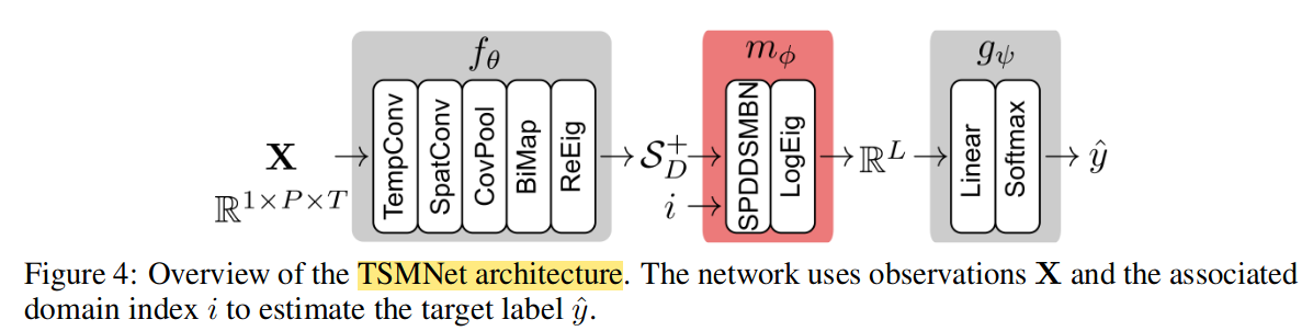
TempConv → SpatConv → CovLayer → BiMap → ReEig → SPDDSMBN → LogEig → Linear softmax.

TempConv: four learned temporal FIR filters.
SpatConv: 40 learned spatio-spectral filters.
CovPool: covariance over time, producing $40 \times 40$ SPD matrices.
BiMap: orthogonally constrained projection from $40 \times 40$ to $20 \times 20$ .
ReEig: floors eigenvalues at $1 0^{- 4}$ .
SPDDSMBN: aligns domain-specific SPD distributions.
LogEig: vectorizes the normalized $20 \times 20$ matrix into 210 norm-preserving upper-triangular features.
Classifier: shared linear softmax layer.

SPDDSMBN maintains a separate SPDMBN instance for domain $i$ :

SPDDSMBN (Z_{j}, i) = SPDMBN_{i} (Z_{j}; G_{ϕ_{i}}, ν_{ϕ_{i}}, ϵ, γ, γ_{train} (k)) .

Each instance tracks separate running Fréchet means and variances for training and testing. A one-step Karcher-flow batch mean updates the running mean along a geodesic, while variance is updated by exponential smoothing. Normalization transports observations from the running Fréchet mean to the identity, rescales their dispersion through a matrix power, and transports them to a parameterized mean:

\tilde{Z}_{j} = Γ_{I \to G_{ϕ}} \circ Γ_{G_{k} \to I} (Z_{j})^{ν_{ϕ} / (ν_{k} + ϵ)} .

TSMNet fixes $G_{ϕ_{i}} = I$ and shares $ν_{ϕ_{i}} = ν_{ϕ}$ across domains. SPDDSMBN followed by LogEig therefore approximates tangent-space mapping at each domain’s Fréchet mean rather than at the identity:

m_{ϕ} (Z) = upper [\frac{ν _{ϕ}}{ν _{k} + ϵ} lo g (G_{k}^{- 1/2} Z G_{k}^{- 1/2})] .

A new SPDMBN instance can be added online for a new domain; the reported experiments are offline.

Model Parameters

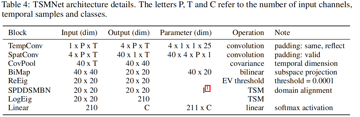
Layer	Input	Output	Parameters
TempConv	$1 \times P \times T$	$4 \times P \times T$	$4 \times 1 \times 1 \times 25$
SpatConv	$4 \times P \times T$	$40 \times 1 \times T$	$40 \times 4 \times P \times 1$
CovPool	$40 \times T$	$40 \times 40$	none
BiMap	$40 \times 40$	$20 \times 20$	$40 \times 20$
ReEig	$20 \times 20$	$20 \times 20$	threshold 0.0001
SPDDSMBN	$20 \times 20$	$20 \times 20$	one shared Fréchet-variance parameter
LogEig	$20 \times 20$	210	none
Linear	210	$C$	$211 \times C$
Implementation names: `n_temp_filters=4`, `temp_kernel_length=25`, `n_spatiotemp_filters=40`, `n_bimap_filters=20`.

Training Parameters

Loss: cross-entropy.
Optimizer: Riemannian Adam.
Learning rate: $1 0^{- 3}$ ; weight decay $1 0^{- 4}$ on unconstrained parameters; $β_{1} = 0.9$ , $β_{2} = 0.999$ .
Batch size: 50 observations (10 observations from each of 5 domains).
Source split: randomized 80% training / 20% validation, stratified across domains and labels.
Epochs: 50 with exhaustive minibatch sampling.
SPDMBN training momentum: $γ_{train} (0) = 1$ , exponentially decayed to $γ_{m i n} = 0.2$ at epoch 40.
Model selection: minimum validation loss over the 50 epochs.
Target adaptation: target-domain normalization statistics computed without labels (Karcher-flow Fréchet mean).

Results

Balanced accuracy (%), mean (SD). Inter-session (IS) and inter-subject (ISub):

Method	4001 IS	4001 ISub	5001 IS	5001 ISub	Lee IS	Lee ISub	Stieger IS	Stieger ISub
FBCSP+SVM	60.6 (4.9)	32.3 (7.3)	81.5 (4.4)	58.6 (13.4)	63.1 (4.2)	63.4 (12.1)	47.5 (7.0)	37.6 (10.5)
TSM+SVM	61.8 (4.1)	34.7 (8.6)	75.7 (5.1)	56.0 (6.0)	62.5 (3.3)	65.3 (13.0)	49.5 (8.1)	40.2 (12.3)
FB+TSM+LR	69.8 (4.8)	36.5 (8.2)	80.9 (6.0)	60.6 (10.9)	65.2 (4.5)	68.5 (12.4)	57.3 (7.3)	40.3 (9.2)
EEGNet	41.8 (5.8)	43.3 (17.0)	72.4 (8.4)	59.2 (9.5)	51.2 (2.7)	69.6 (13.8)	58.3 (7.9)	43.1 (11.0)
ShConvNet	51.3 (2.3)	42.2 (16.2)	74.1 (4.2)	58.7 (5.8)	57.8 (4.0)	68.5 (13.6)	60.1 (6.6)	42.2 (10.4)
FBCSP+DSS+LDA	71.3 (1.8)	48.3 (14.3)	84.6 (4.8)	67.7 (14.3)	66.8 (4.1)	68.7 (13.8)	59.4 (6.6)	48.2 (13.4)
URPA+MDM	59.5 (2.7)	46.8 (14.6)	79.2 (4.6)	70.3 (16.1)	63.8 (4.2)	66.7 (12.3)	47.0 (6.6)	38.7 (10.4)
SPDOT+TSM+SVM	66.8 (3.8)	38.6 (8.6)	77.5 (2.9)	63.3 (8.1)	65.6 (4.2)	65.4 (10.5)	50.3 (5.8)	42.1 (10.5)
EEGNet+DANN	50.0 (7.7)	45.8 (18.0)	71.6 (5.3)	63.7 (11.1)	55.4 (4.4)	69.4 (13.1)	60.1 (6.9)	43.6 (10.7)
ShConvNet+DANN	51.6 (3.2)	42.2 (13.6)	74.1 (4.0)	64.2 (11.6)	59.1 (3.4)	66.0 (12.4)	61.3 (6.0)	43.1 (11.5)
TSMNet	69.0 (3.6)	51.6 (16.5)	85.8 (4.3)	77.0 (13.7)	68.2 (4.1)	74.6 (14.2)	64.8 (6.8)	48.9 (14.3)

Method	Lehner IS	Hehenberger IS	Hinss IS	Hinss ISub
FBCSP+SVM	68.9 (6.0)	52.5 (7.1)	43.7 (8.2)	45.6 (6.5)
EEGNet	49.6 (6.4)	48.2 (6.3)	46.3 (10.1)	47.8 (5.1)
FBCSP+DSS+LDA	77.1 (8.4)	56.4 (5.3)	47.1 (7.4)	48.4 (9.0)
TSMNet	77.7 (10.0)	57.8 (5.8)	54.7 (7.3)	52.4 (8.8)

Ablation across five MI datasets and 138 subjects, inter-session transfer (Δ balanced accuracy; fit time for 50 epochs):

SPD geometry	DSBN	BN method	Δ bal. acc.	Fit time
yes	yes	SPDMBN	reference	16.9 (1.0) s
yes	yes	SPDBN	-1.6 (2.2)	20.3 (1.6) s
yes	no	SPDMBN	-3.9 (4.4)	11.3 (0.5) s
no	yes	MBN	-4.5 (3.8)	6.6 (0.2) s
no	no	MBN	-6.9 (4.8)	4.4 (0.1) s

Notes

Follow-up: SPDIM (Li et al. 2024) reuses the TSMNet architecture on Zhou2016 (3 classes, sessions as domains, leave-one-group-out, 80/20 stratified train/val, 100 epochs, Riemannian ADAM — a different schedule from TSMNet’s 50 epochs) and adds an SPD invariant bias (SPDIM-bias 84.1% cross-session / 80.4% cross-subject under 0.2 label ratio).

Lucas Heck's Notes

Explorer

TSMNet